Lovecraft in words
tags:
In one of the Java courses I took on Coursera, a simple exercise consists in counting the occurrences of the words in a file. The examples we used were plays from Shakespeare and while I’ve read a few of them I prefer Lovecraft and Python.
The idea is simple:
- we read a file
- split it into words
- count the occurrences of the words that are not common english words.
We’ll repeat this operation for many short stories of Lovecraft and we’ll visualize the most frequent words of each short story. Hopefully, this should give us an idea of what each one is about.
This post was created using the Jupyter Notebook with a few libraries:
%matplotlib inline
import os
from collections import defaultdict
import time
import re
from fntools import count
import matplotlib.pyplot as plt
import pandas as pd
import matplotlib
matplotlib.style.use('ggplot')
from wordcloud import WordCloud
from itertools import repeat
Counting the relevant words
Here are the functions we’ll need to count the words.
def count_words_frequency(inputfile, excluded=[]):
    """Count the frequency of the words in the inputfile

    Excluded words can be specified with the keywords `excluded`.

    """
    frequencies = defaultdict(int)
    with open(inputfile) as f:
        for line in f:
            for word in line.split():
                word = word.lower().strip()
                word = re.sub("[^a-z]", "", word)
                if len(word) > 0 and word not in excluded:
                    frequencies[word] += 1
    return frequencies


def count_total_words(frequencies):
    """Count the total number of words from the given frequency table"""
    return sum(count for word, count in frequencies.items())
In order to exclude the words that occur frequently in the english language and that would distort the results I used the 10000 most common english words as determined by n-gram frequency analysis of the Google’s Trillion Word Corpus.
CURRENT_DIR = os.path.expanduser("~/Dropbox/Projects/Lovecraft")
ENGLISH_WORDS_FILE = CURRENT_DIR + "/data/google-10000-english.txt"

def get_most_common_english_words(max_word_count=1000):
    """Return a list of the most common english words.

    The maximum number of words can be specified with `max_word_count`.
    The maximum number of available words is 10000.

    """
    most_common_english_words = []
    n = 0
    with open(ENGLISH_WORDS_FILE) as f:
        while n < max_word_count:
            most_common_english_words.append(f.readline().strip())
            n += 1
    return most_common_english_words
Now the processing part. There’s a bit of calibration to do to determine the most common english words we consider. Indeed if we exclude the 10000 most common words, we’ll have mainly the names of the protagonists, or rare words left. In some cases, this may not tell us much about what is happening but rather who is in the story. On the other hand if we choose a lower value we may get some useful words but other may be irrelevant. After some tests, I chose to exclude the first 5000 most common words. Note that we could adapt this value to each short story but, for the sake of simplicity, we’ll stick to 5000 for the 6 texts we’ll analyze.
Then let’s apply our function for counting the frequency of the words (count_words_frequency) and store them in a pandas.DataFrame:
filenames = ("cthulhu.txt", "mountains_of_madness.txt", "the_unnamable.txt", "charles_dexter_ward.txt",
         "wall_of_sleep.txt", "erich_zann.txt")

english_words = get_most_common_english_words(5000)

words_frequency = {}
total_words = {}
dfs = {}

for filename in filenames:
    inputfile = os.path.join(CURRENT_DIR, "data", filename)
    name = filename[:-4]
    print 'Reading %s...' % filename
    words_frequency[name] = count_words_frequency(inputfile, english_words)
    total_words[name] = count_total_words(words_frequency[name])
    dfs[name] = pd.DataFrame(words_frequency[name].items(), columns=('word', 'frequency'))
Let’s look at the example of ‘The Call of Cthulhu’ and see what the 3 most frequent words are:
dfs['cthulhu'].sort_values(by='frequency', ascending=False).head(3)
| word | frequency |
|---|---|
| cult | 30 |
| johansen | 23 |
| cthulhu | 22 |
From what we see, ‘The Call of Cthulhu’ is mainly about a cult, a person called Johansen and the famous Cthulhu. Sounds right!
Visualization
We visualize the most frequent words with a word cloud using the word_cloud package:
def plot_word_cloud(data, n=20):
    """Plot the n most frequent words with wordcloud"""
    text = []
    for word, freq in data:
        text.extend(list(repeat(word, freq)))

    text = ','.join(text)
    # Generate a word cloud image
    wordcloud = WordCloud(background_color='white').generate(text)

    # Display the generated image:
    # the matplotlib way
    plt.figure(figsize=(8, 6))
    plt.imshow(wordcloud)
    plt.axis("off")
    return plt
The call of Cthulhu
cthulhu = dfs['cthulhu'].sort_values(by='frequency', ascending=False).head(10)
cthulhu
| word | frequency |
|---|---|
| cult | 30 |
| johansen | 23 |
| cthulhu | 22 |
| uncle | 21 |
| legrasse | 20 |
| wilcox | 19 |
| angell | 13 |
| whilst | 12 |
| manuscript | 11 |
| basrelief | 11 |
plot_word_cloud(cthulhu.values);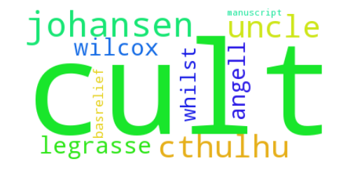
The mountains of madness
mountains_of_madness = dfs['mountains_of_madness'].sort_values(by='frequency', ascending=False).head(10)
mountains_of_madness
| word | frequency |
|---|---|
| danforth | 53 |
| antarctic | 48 |
| vast | 43 |
| sculptures | 41 |
| specimens | 37 |
| monstrous | 31 |
| curious | 31 |
| carvings | 30 |
| abyss | 29 |
| peaks | 28 |
plot_word_cloud(mountains_of_madness.values);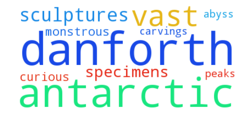
The unnamable
the_unnamable = dfs['the_unnamable'].sort_values(by='frequency', ascending=False).head(10)
the_unnamable
| word | frequency |
|---|---|
| manton | 13 |
| unnamable | 9 |
| attic | 9 |
| tomb | 7 |
| deserted | 7 |
| whispered | 5 |
| slab | 4 |
| spectral | 4 |
| legends | 3 |
| slate | 3 |
plot_word_cloud(the_unnamable.values);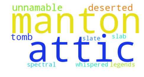
The case of Charles Dexter Ward
charles_dexter_ward = dfs['charles_dexter_ward'].sort_values(by='frequency', ascending=False).head(10)
charles_dexter_ward| word | frequency |
|---|---|
| willett | 169 |
| curwen | 158 |
| ye | 87 |
| wards | 52 |
| pawtuxet | 50 |
| curwens | 43 |
| providence | 37 |
| weeden | 35 |
| capt | 33 |
| curious | 33 |
plot_word_cloud(charles_dexter_ward.values);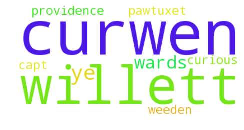
Beyond the wall of sleep
wall_of_sleep = dfs['wall_of_sleep'].sort_values(by='frequency', ascending=False).head(10)
wall_of_sleep| word | frequency |
|---|---|
| slater | 25 |
| waking | 6 |
| decadent | 5 |
| cosmic | 5 |
| cannot | 4 |
| couch | 4 |
| ethereal | 4 |
| valleys | 4 |
| oppressor | 4 |
| luminous | 4 |
plot_word_cloud(wall_of_sleep.values);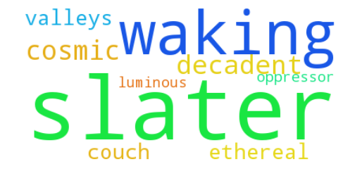
The music of Erich Zann
erich_zann = dfs['erich_zann'].sort_values(by='frequency', ascending=False).head(10)
erich_zann
| word | frequency |
|---|---|
| zann | 17 |
| viol | 13 |
| rue | 11 |
| dauseil | 11 |
| garret | 8 |
| erich | 8 |
| dumb | 6 |
| zanns | 5 |
| strains | 4 |
| shutter | 4 |
plot_word_cloud(erich_zann.values);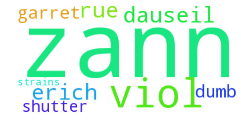
Conclusion
From the results, we clearly see the topics Lovecraft treated in his stories: strange cults, dreams, madness and powerless men facing terrifying creatures. From a technical point of view, this approach is a bit simplistic but it’s a good approximation. This study could be improved with natural language processing. Instead of creating a meaning from a list of words, we could analyze the sentiments in the each short story.